Intro to Stats
Introduction to Basic Stats in R
Code from session
#Independent-Samples T-test
#Create variables
Women = c(99, 85, 78, 93, 95, 87)
Men = c(72, 75, 70, 68, 70, 80)
#T-test to see if men and women's scores significantly differ
t.test(Women,Men,alternative="two.sided")
##
## 	Welch Two Sample t-test
##
## data:  Women and Men
## t = 4.7332, df = 7.9586, p-value = 0.001498
## alternative hypothesis: true difference in means is not equal to 0
## 95 percent confidence interval:
##   8.71012 25.28988
## sample estimates:
## mean of x mean of y
##      89.5      72.5
#One-sample t-test to see if women scored significantly lower than 95% on the test
t.test(Women, alternative = "less", mu = 95)
##
## 	One Sample t-test
##
## data:  Women
## t = -1.7644, df = 5, p-value = 0.06897
## alternative hypothesis: true mean is less than 95
## 95 percent confidence interval:
##      -Inf 95.78122
## sample estimates:
## mean of x
##      89.5
#One-way analysis of variance
#Read sample pain score data into R
pain = c(4, 5, 4, 3, 2, 4, 3, 4, 4, 6, 8, 4, 5, 4, 6, 5, 8, 6, 6, 7, 6, 6, 7, 5, 6, 5, 5)
gender = c("F", "F", "F", "M", "M", "M", "M", "F", "F", "M", "M", "F", "F", "F", "M", "F", "M", "M", "M", "F", "F", "F", "F", "M", "F", "M", "M")
#Code the data according to which drug is associated with the score
drug = c(rep("A",9), rep("B",9), rep("C",9))
#Create data frame with pain scores, coded by which drug the patient took
migraine = data.frame(pain,drug)
#Look at our data frame
migraine
##    pain drug
## 1     4    A
## 2     5    A
## 3     4    A
## 4     3    A
## 5     2    A
## 6     4    A
## 7     3    A
## 8     4    A
## 9     4    A
## 10    6    B
## 11    8    B
## 12    4    B
## 13    5    B
## 14    4    B
## 15    6    B
## 16    5    B
## 17    8    B
## 18    6    B
## 19    6    C
## 20    7    C
## 21    6    C
## 22    6    C
## 23    7    C
## 24    5    C
## 25    6    C
## 26    5    C
## 27    5    C
#Run a one-way ANOVA
results = aov(pain ~ drug, data=migraine)
summary(results)
##             Df Sum Sq Mean Sq F value   Pr(>F)
## drug         2  28.22  14.111   11.91 0.000256 ***
## Residuals   24  28.44   1.185
## ---
## Signif. codes:  0 '***' 0.001 '**' 0.01 '*' 0.05 '.' 0.1 ' ' 1
#Post hoc analysis using Tukey's HSD
TukeyHSD(results, conf.level = 0.95)
##   Tukey multiple comparisons of means
##     95% family-wise confidence level
##
## Fit: aov(formula = pain ~ drug, data = migraine)
##
## $drug
##          diff        lwr      upr     p adj
## B-A 2.1111111  0.8295028 3.392719 0.0011107
## C-A 2.2222222  0.9406139 3.503831 0.0006453
## C-B 0.1111111 -1.1704972 1.392719 0.9745173
#Add column full of gender info to migraine dataset
migraine$gender <- c("F", "F", "F", "M", "M", "M", "M", "F", "F", "M", "M", "F", "F", "F", "M", "F", "M", "M", "M", "F", "F", "F", "F", "M", "F", "M", "M")
migraine
##    pain drug gender
## 1     4    A      F
## 2     5    A      F
## 3     4    A      F
## 4     3    A      M
## 5     2    A      M
## 6     4    A      M
## 7     3    A      M
## 8     4    A      F
## 9     4    A      F
## 10    6    B      M
## 11    8    B      M
## 12    4    B      F
## 13    5    B      F
## 14    4    B      F
## 15    6    B      M
## 16    5    B      F
## 17    8    B      M
## 18    6    B      M
## 19    6    C      M
## 20    7    C      F
## 21    6    C      F
## 22    6    C      F
## 23    7    C      F
## 24    5    C      M
## 25    6    C      F
## 26    5    C      M
## 27    5    C      M
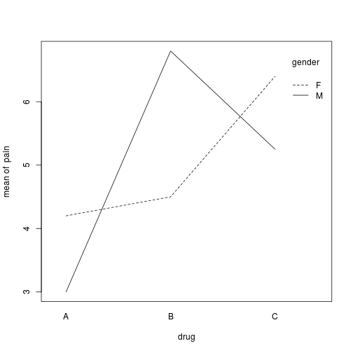
#Run two-way ANOVA using gender and drug as factors
results = aov(pain ~ drug*gender, data=migraine)
summary(results)
##             Df Sum Sq Mean Sq F value   Pr(>F)
## drug         2 28.222  14.111  28.088 1.16e-06 ***
## gender       1  0.002   0.002   0.004    0.952
## drug:gender  2 17.893   8.946  17.808 3.00e-05 ***
## Residuals   21 10.550   0.502
## ---
## Signif. codes:  0 '***' 0.001 '**' 0.01 '*' 0.05 '.' 0.1 ' ' 1
#Post hoc analysis on two-way ANOVA
TukeyHSD(results, conf.level = 0.95)
##   Tukey multiple comparisons of means
##     95% family-wise confidence level
##
## Fit: aov(formula = pain ~ drug * gender, data = migraine)
##
## $drug
##          diff       lwr       upr     p adj
## B-A 2.1111111  1.268923 2.9532993 0.0000084
## C-A 2.2222222  1.380034 3.0644104 0.0000040
## C-B 0.1111111 -0.731077 0.9532993 0.9410333
##
## $gender
##            diff        lwr       upr     p adj
## M-F -0.01648352 -0.5842182 0.5512512 0.9524246
##
## $`drug:gender`
##          diff        lwr         upr     p adj
## B:F-A:F  0.30 -1.1875023  1.78750227 0.9873049
## C:F-A:F  2.20  0.7975694  3.60243059 0.0009237
## A:M-A:F -1.20 -2.6875023  0.28750227 0.1619424
## B:M-A:F  2.60  1.1975694  4.00243059 0.0001207
## C:M-A:F  1.05 -0.4375023  2.53750227 0.2752703
## C:F-B:F  1.90  0.4124977  3.38750227 0.0074874
## A:M-B:F -1.50 -3.0679651  0.06796506 0.0660199
## B:M-B:F  2.30  0.8124977  3.78750227 0.0010862
## C:M-B:F  0.75 -0.8179651  2.31796506 0.6700989
## A:M-C:F -3.40 -4.8875023 -1.91249773 0.0000064
## B:M-C:F  0.40 -1.0024306  1.80243059 0.9441652
## C:M-C:F -1.15 -2.6375023  0.33750227 0.1947322
## B:M-A:M  3.80  2.3124977  5.28750227 0.0000011
## C:M-A:M  2.25  0.6820349  3.81796506 0.0024216
## C:M-B:M -1.55 -3.0375023 -0.06249773 0.0379545
#Plot the interaction for our two-way ANOVA
interaction.plot(drug, gender, pain)
#Create bachelor dataset for correlation demo
weeks = c(8,7,6,5,4,4,3,3,3,2,2,2,1,1,1,1,1,1,1,1,1,1,1,1,1,1)
age = c(24,23,25,24,23,22,27,28,23,30,27,30,24,27,29,30,27,29,25,34,27,22,25,28,28,23)
bachelor = data.frame(weeks, age)
bachelor
##    weeks age
## 1      8  24
## 2      7  23
## 3      6  25
## 4      5  24
## 5      4  23
## 6      4  22
## 7      3  27
## 8      3  28
## 9      3  23
## 10     2  30
## 11     2  27
## 12     2  30
## 13     1  24
## 14     1  27
## 15     1  29
## 16     1  30
## 17     1  27
## 18     1  29
## 19     1  25
## 20     1  34
## 21     1  27
## 22     1  22
## 23     1  25
## 24     1  28
## 25     1  28
## 26     1  23
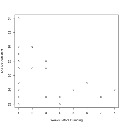
#Run test of correlation on bachelor data - default method is Pearson correlation
cor.test(bachelor$weeks, bachelor$age)
##
## 	Pearson's product-moment correlation
##
## data:  bachelor$weeks and bachelor$age
## t = -2.3978, df = 24, p-value = 0.02463
## alternative hypothesis: true correlation is not equal to 0
## 95 percent confidence interval:
##  -0.70663528 -0.06298623
## sample estimates:
##        cor
## -0.4396126
plot(bachelor$weeks, bachelor$age, xlab="Weeks Before Dumping", ylab="Age of Contestant")
#Supplemental: Another kind of post hoc test (pairwise t-tests with a bonferroni correction) on the migraine dataset
pairwise.t.test(pain, drug, p.adjust="bonferroni")
##
## 	Pairwise comparisons using t tests with pooled SD
##
## data:  pain and drug
##
##   A       B
## B 0.00119 -
## C 0.00068 1.00000
##
## P value adjustment method: bonferroni
#Supplemental: Another way to do a t-test on the migraine dataset
with(migraine, t.test(pain[drug == "A"], pain[drug == "B"]))
##
## 	Welch Two Sample t-test
##
## data:  pain[drug == "A"] and pain[drug == "B"]
## t = -3.6909, df = 12.896, p-value = 0.002751
## alternative hypothesis: true difference in means is not equal to 0
## 95 percent confidence interval:
##  -3.3478073 -0.8744149
## sample estimates:
## mean of x mean of y
##  3.666667  5.777778
Python-ized version (courtesy of @QuLogic)